

Volume 4, Issue 4 (December 2019)
J Environ Health Sustain Dev 2019, 4(4): 903-912 |
Back to browse issues page


Download citation:
BibTeX | RIS | EndNote | Medlars | ProCite | Reference Manager | RefWorks
Send citation to:


BibTeX | RIS | EndNote | Medlars | ProCite | Reference Manager | RefWorks
Send citation to:
Almodaresi S A, Mohammadrezaei M, Dolatabadi M, Nateghi M R. Qualitative Analysis of Groundwater Quality Indicators Based on Schuler and Wilcox Diagrams: IDW and Kriging Models. J Environ Health Sustain Dev 2019; 4 (4) :903-912
URL: http://jehsd.ssu.ac.ir/article-1-190-en.html
URL: http://jehsd.ssu.ac.ir/article-1-190-en.html


Department of GIS & RS, Yazd Branch, Islamic Azad University, Yazd, Iran.
Full-Text [PDF 784 kb]
(876 Downloads)
| Abstract (HTML) (1842 Views)
.png)
Figure 1: Location of study area of Yazd-Ardakan-Mehriz
Figure 2: Contour plot of the A) SO4, B) TDS, C) TH, D) Mg, E) Cl, F) Ca, G) HCO3, and H) of the
quality of drinking water based on Schuler parameters.
Figure 3: A) Contour plot of the EC B) SAR of the groundwater in Yazd-Ardakan-Mehriz.
.png)
Figure 4: Contour plot of the groundwater quality for agricultural irrigation.
Full-Text: (991 Views)
Qualitative Analysis of Groundwater Quality Indicators Based on Schuler and Wilcox Diagrams: IDW and Kriging Models
Seyed Ali Almodaresi 1*, Mohsen Mohammadrezaei 1, Maryam Dolatabadi 2, Mohammad Reza Nateghi 3
1 Department of GIS & RS, Yazd Branch, Islamic Azad University, Yazd, Iran.
2 Environmental Science and Technology Research Center, Department of Environmental Health Engineering, Shahid Sadoughi University of Medical Sciences, Yazd, Iran.
3 Department of Chemistry, Islamic Azad University, Yazd, Iran.
| A R T I C L E I N F O | ABSTRACT | |
| ORIGINAL ARTICLE | Introduction: It is generally accepted that groundwater is one of the most vital sources of water for drinking use in cities and rural areas. The water drawn from these sources should be sanitary, have low soluble substances, and be free of any pathogens and microorganisms. Materials and Methods: In this study, 90 wells were sampled with proper dispersion over the study area to achieve suitable estimation accuracy. Results: The assessments made based on 10-year averages of water quality in the studied plain showed that according to the Schuler and Wilcox criteria of water quality for drinking and agricultural use, the northern and southern parts of the plain have unsuitable water quality compared to central parts. Interpolation RMSE value of the Inverse Distance Weighting (IDW) model for SO4-, TDS, TH, Mg2+, Cl-, Ca2+ and HCO3- were 8.46, 2615, 246, 6.8, 38.9, 8.3 1.16 also 8.4, 2628, 750.9, 7.0, 39.8, 8.1, 8.1 (mg L-1) for Kriging, respectively. Conclusion: The cause of low groundwater quality in northern regions is the high rate of SO4-, TH, Cl-, and TDS, which are of the most important determinants of water quality for drinking. The examination of samples in the assessment of water quality for agricultural use clearly showed a higher value of EC compared to SAR. |
|
| Article History: Received: 12 August 2019 Accepted: 20 October 2019 |
||
| *Corresponding Author: Seyed Ali Almodaresi Email: Almodaresi@iauyazd.ac.ir Tel: +989131526455 |
||
| Keywords: Schuler Diagram, Wilcox Diagram, IDW and Kriging Models, Drinking Water, Ardakan Mehriz plain. |
Citation: Almodaresi SA, Mohammadrezaei M, Dolatabadi M, et al. Qualitative Analysis of Groundwater Quality Indicators Based on Schuler and Wilcox Diagrams: IDW and Kriging Models. J Environ Health Sustain Dev. 2019; 4(4): 903-12.
Introduction
Geographic information systems are widely used in the monitoring and qualitative classification of river water and facilitate large scale analysis of data. Using this system, it is possible to devise more effective management plans by identifying important demographic, industrial and agricultural centers and estimating the pollution load in combination with other information. Arid areas suffer from water scarcity because of low annual rainfall and high evaporation, which sometimes reaches as high as 40 times the precipitation 1, 2. Groundwater is one of the most important sources of drinking water for urban and rural settlements. The water drawn from these sources should be completely hygienic, have low soluble substances, and be free of any pathogens. Research has shown that bedrock is one of the key factors affecting the chemical composition of water 3, 4. According to Gibbs, the chemical composition of surface water is controlled by three major factors: rock dominance, precipitation, and evaporation-crystallization process. However, the Gibbs model ignores the non-uniform distribution of water on the ground at different scales, which many consider a weak point. In World Health Organization (WHO) and United Nations Environment Programme (UNEP) reports, surface water and groundwater compositions are considered dependent on natural factors (geology, topography, meteorology, hydrology, and biology) in the drainage basin, and seasonal variations in water runoff volume, weather conditions, and surface water levels. Human activities have also a significant impact on the quality of water. Some of these effects are the result of hydrological changes such as the construction of dams, drying of wetlands, and deviation in flow path 5-7.
The classification of water quality for agricultural use was performed using the Wilcox diagram. This diagram determines the quality of water for agriculture use based on two parameters: Electrical Conductivity (EC) and Sodium Absorption Ratio (SAR). The horizontal axis represents EC in micromhos per cm and the vertical axis represents the SAR value. Sodium Absorption Ratio, or SAR, is the ratio of sodium ions in a water sample to calcium and magnesium ions 8, 9:
If SAR is less than 4, then the soil has an appropriate amount of sodium. If this ratio is greater than 8, the soil exhibits decreases permeability and changes in texture. And if this ratio is greater than 13, then the soil is sodic. In the standards of water quality for agricultural use, SAR values are classified into 4 groups: 1- Less than 10 (low and good) 2- Values between 11-18 (moderate) 3- Values between 19-26 (high) and 4- Values greater than 27 (Very high). EC values are also classified into 4 groups: 1- values between 100-250 (low) 2- values between 251-750 (moderate) 3- values between 751-2251 (high) and 4- values greater than 2251 (very high).
Maghami et al. in the study tried to evaluate water quality using different interpolation methods and Geographic Information System (GIS). In this study, 27 wells in Abadeh zone were studied. Interpolation methods (Kriging with semi-linear, circular, spherical, Inverse Distance Weighting (IDW), Spline, Gaussian and exponential variograms) and GIS were used for zoning the water quality of the study area. The results of this study showed that among the above-mentioned methods, Kriging with exponential and circular semivariograms are the most suitable methods for interpolation and finally zoning of drinking water quality 10.
Nowadays, interpolation has extensive use in many research and scientific projects for estimating development in the study area, urban and rural planning, and other areas. The use of interpolation models depends on access to known data in the study area 11, 12. Therefore, mathematical models and methods can be employed for more accurate estimation. The most accurate method based on interpolation operations is geostatistics, which has managed to increase the accuracy of estimates through scientific models. In this study, the drinking water and groundwater quality in Ardakan Mehriz plain is studied based on Schuler and Wilcox criteria in four steps:
- Evaluation and sampling of 93 wells in the plain and identifying the elements that affect the water quality assessment.
- Kriging interpolation for each of the elements that affect the water quality assessment (obtained from the previous step) according to the relevant contour plot using the inverse distance interpolation method and by an evaluation based on mean squared error.
- Determining the range of water quality by comparing the data obtained from the previous steps using the Schuler diagram, which classifies water into six categories: good, acceptable, moderate, unsuitable, quite unpleasant, and non-potable.
- Zoning the area based on the effective parameters with the help of the Wilcox diagram.
Materials and Methods
Study Area
Ardakan-Mehriz plain is the wide drainage basin of Yazd province in Iran. This plain is located between 53°24ʹ42″ and 54°56ʹ42″ eastern longitudes and 31°13ʹ30″ and 32°36ʹ6″ northern latitudes in an area of about 10741 km2. This plain is the largest and the most important aquifer of the province and is used for agriculture, drinking, and industrial purposes in Yazd-Ardakan-Mehriz (Figure 1). In this study, Yazd-Ardakan-Mehriz aquifer is zoned in terms of groundwater quality using Schuler and Wilcox criteria in the GIS environment. In addition, the effect of spatial and temporal variations on qualitative characteristics of the aquifer groundwater is analyzed using geostatistical methods. In this study, the time range of ten years’ period was studied from 2007 to 2017. The information required to assess water quality was obtained from Yazd Water and Wastewater Company. The experiments related to the investigation were performed in triplicate and repeated three times and the average data were presented. Samples were collected from the sampling time until they were transported to the laboratory in the ice which were stored at a temperature of 2 ° C.
Figure 1: Location of study area of Yazd-Ardakan-Mehriz
Data and Method
Geostatistics is one of the best applications of interpolation operation, which has been able to improve the accuracy of estimation through scientific models. Accordingly, geostatistics can be used to convert observations into data. In the GIS environment, geographical data are divided into two types based on the analytical methods: discrete data and continuous data. Discrete data are mostly categorical data, meaning that in essence they have precisely definable boundaries and can be stored as a raster or vector, (e.g. lake, building, or road). Continuous data are continuous in nature, meaning that every point on the ground will have a degree of the property or variable they describe. Liquids belong to the latter group, but also have a direction and can be measured at any point. Because of their continuity, continuous data cannot be measured at all levels and have to be sampled. Interpolation is the estimation of continuous variables in the non-sampled areas within an area with scattered observation points. The output of the interpolation can be used as a plot or layer in the GIS analysis. There are many methods for interpolation of continuous data, but this study used two methods for this purpose: IDW and Kriging models.
Inverse Distance Weighting (IDW)
In IDW model, it is assumed that the effectiveness of the continuous variable decreases with the distance from the unknown point, therefore the distance is used as the weight of the known variable in the estimation of unmeasured points. This method is called Inverse Distance Weighting because as the distance from the unknown point increases, the weight decreases 13, 14. The effect of the intensity of spatial dependence of data can be applied to the formulation by raising the power of the inverse distance. The square of the inverse distance is a popular choice for this purpose. In this method, the target range is transformed into a matrix with cells of equal size. The spatial coordinates of this matrix and the measurement unit are known. For example, a matrix may have 50×50 m2 cells. In this grid, the value of the variable is known in some cells and unknown in others. Each unknown value is estimated using the values of neighboring cells within a given radius using the following equation 14, 15.
Where the value is measured at the ith position and is the weight measured at the ith position. S0 is the position of the estimated value and N is the number of measured or known points. is a function of the distance between points. The dependence of the unknown cells on known cells is adjusted by the power of the inverse distance. The appropriate power ( ) is determined based on the Root Mean Square Prediction Error (RMSPE). The best value for is the one that yields the best estimations of unknown cells, or in the other words minimizes the prediction error. The points on the curve represent different RMSPE values obtained with different values. The minimum value of RMSPE on the curve gives the best power for the IDW model.
When this power is zero ( ), the impact of the distance is uniform and the unknown value is obtained by averaging the values of neighboring points. But as this power increases, the impact of distance also increases, and closer cells gain a higher weight in the formulation.
In the IDW model, it is typical to use greater than 1, such as 2, which is why it is also called squared inverse distance. In the IDW model Neighborhood can be defined in two ways. The fixed search radius method assumes a circle around the unknown point and calculates this value based on the points positioned within the circle. In other words, to calculate the unknown point, the distance of each of the points inside the circle will be measured, the measured distances will be raised to second order, and the results will be averaged. The value is actually the weight given to the distances. This means to increase the effect of distance, so the value of is increased. The size of the search radius depends on the distance between the points and the manner of changes in the continuous variable. If the variable changes irregularly, one can use the nearest neighbor’s method instead of the fixed search radius. This method is similar to the previous method, with the difference that interpolation is performed with the minimum number of neighbors. In other words, the neighborhood is defined with the number of neighbors 16, 17.
Kriging Model
The Kriging method is the most important and extensively used method of statistical interpolation. Kriging is an advanced interpolation method most suitable for data with well-defined local trends. The Kriging method operates based on the minimum variance of estimation, and its error is a function of variogram characteristics (spatial structure) 18, 19. As long as variographic analysis and variogram model are sufficiently accurate, the kriging method will be accurate as well. The Kriging model is generally similar to the IDW model 20, 21:
Where is the value measured at the ith is position and is the weight measured at the ith position. S0 is the position of the estimated value and N is the number of measured or known points. In the IDW model, is only a function of distance, but in the kriging model, the weight also depends on the spatial structure of the points. Accordingly, the Kriging model is a good interpolation model for geostatistical purposes. The kriging model operates based on the regionalized variable theory, where the value of each point in space is a function of its coordinates. Therefore, the variation of the regionalized variable in space is decomposed into 4 components.
Where m(x) is the function giving the structural element Z at point x, is the function describing the random component, which is spatially dependent and locally variable, and is the residue or random error, which has a zero mean and constant variance and is spatially independent. In a semi-variogram, every two samples can be paired with each other, as there is a known distance between them. Therefore, for better management of the semivariogram, instead of drawing all pairs, they are grouped based on their distance. For example, all pairs that have a distance of more than 40 meters and less than 50 meters from each other can be categorize in one group. After drawing the semivariograms, a suitable regression model will be fitted into it 22, 23.
Results
Accuracy evaluation method
Different interpolation methods are evaluated using the cross-validation method. In this method, a point will be temporarily removed and will then be estimated based on other points using interpolation. The removed value will then be returned and this process will be repeated for all remaining points. In the end, a table with two columns, one for actual values and the other for estimated values will be created. Having these two values, Mean Absolute Error (MAE) and Mean Bias Error (MBE) of the model can be measured. The closer the MAE and MBE values are to zero, the more accurate is the model. Other measures for assessing the accuracy of interpolation methods are the Root Mean Square Error (RMSE) and the correlation coefficient (R2) between observed and measured values. Greater RMSE values represent a higher error, but in the case of R2, greater values indicate higher statistical accuracy 24, 25 (Table 1).
These measures are calculated as follows:
Table 1: Comparison between the RMSE value of the Kriging model and the IDW model
| RMSE of Kriging | RMSE of IDW | Interpolation |
| 8.45 | 8.46 | SO4- (mg L-1) |
| 2628.92 | 2615.69 | Total dissolved solids ( mg L-1) |
| 750.93 | 746.27 | TH (mg L-1) |
| 7.01 | 6.83 | Mg2+ (mg L-1) |
| 39.80 | 38.90 | Cl- (mg L-1) |
| 8.14 | 8.29 | Ca2+ (mg L-1) |
| 8.14 | 1.16 | HCO3- (mg L-1) |
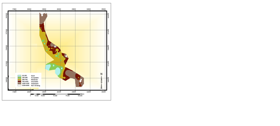
Using the samples taken in a 10-year period, the contour plots were obtained for each parameter, and the water quality plots were drawn accordingly. According to Schuler criteria for drinking water quality, it seems that central and southwestern parts of the studied region have good and acceptable water quality, but southeastern and northern parts have a low water quality, which fall into unsuitable and even unpleasant category (Figure 2).
|
A
.png) |
|
B
.png) |
|
D
.png) |
|
C
.png) |
|
E
 |
|
F
 |
|
H
 |
|
G
 |
Figure 2: Contour plot of the A) SO4, B) TDS, C) TH, D) Mg, E) Cl, F) Ca, G) HCO3, and H) of the
quality of drinking water based on Schuler parameters.
Water quality assessment for agricultural use
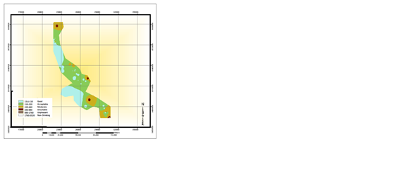
The present study used this classification with the Wilcox criteria. The figures below show the zone plots related to SAR and EC and the results regarding the water quality for irrigation based on the Wilcox diagram and criteria 26-28 (Figure 3, 4).
The present study used this classification with the Wilcox criteria. The figures below show the zone plots related to SAR and EC and the results regarding the water quality for irrigation based on the Wilcox diagram and criteria 26-28 (Figure 3, 4).
|
B
 |
|
A
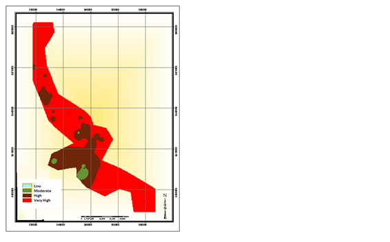 |
Figure 3: A) Contour plot of the EC B) SAR of the groundwater in Yazd-Ardakan-Mehriz.
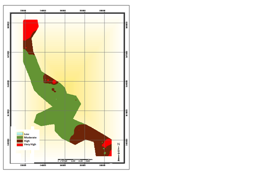
Figure 4: Contour plot of the groundwater quality for agricultural irrigation.
Having the parameters affecting the water quality for agricultural use based on the Wilcox diagram, the EC and SAR plots were drawn and the results were obtained accordingly. The obtained results showed that in the northern and the southeastern parts of the plain, water quality is unacceptable even for agricultural use. However, water in the central parts of the plain has a suitable quality for irrigation 26, 27.
Discussion
It should be noted that given the sampling of 90 wells and the proper dispersion of these samples, good accuracy in quality estimation was achieved. The assessments made based on 10-year averages of water quality in the studied plain show that according to the Schuler and Wilcox criteria of water quality for drinking and agricultural use, the northern and southern parts of the plain have unsuitable water quality compared to central parts. According to the contour plot, the reason for this poor quality in the northern regions is the high rate of SO4, TH, Cl, and TDS, which are of the most important determinants of water quality for drinking use. The examination of samples in the assessment of water quality for agricultural use clearly showed the higher value of EC compared to SAR.
Conclusion
According to examinations of this study, it can be concluded that groundwater quality in the central parts of the plain has suitable quality for irrigation, however; groundwater quality in the northern and southeastern parts of the plain is unacceptable even for agricultural use. The IDW model is better than the Kriging model for analyzing the groundwater quality of the study area. Using geostatistics and GIS, it is possible to identify areas with suitable water quality for agriculture and drinking in the study area. The trends of spatial variations of TDS, pH, EC, and NO3- change along the plain.
Acknowledgments
We would like to express our gratitude to Yazd Branch, Islamic Azad University for supporting this research.
Funding
This research was funded by the Deputy
of Research and Technology (Grant: 11052881201003) at Yazd Branch, Islamic Azad University, Iran.
Conflict of interest
The authors of this article declare that there is no conflict of interest.
This is an Open Access article distributed in accordance with the terms of the Creative Commons Attribution (CC BY 4.0) license, which permits others to distribute, remix, adapt, and build upon this work for commercial use.
References
- Biglari H, Chavoshani A, Javan N, et al. Geochemical study of groundwater conditions with special emphasis on fluoride concentration, Iran. Desalin Water Treat. 2016;57(47):22392-9.
- Rahmati O, Pourghasemi HR, Melesse AM. Application of GIS-based data driven random forest and maximum entropy models for groundwater potential mapping: a case study at Mehran Region, Iran. Catena. 2016;137:360-72.
- Izady A, Davary K, Alizadeh A, et al. Groundwater conceptualization and modeling using distributed SWAT-based recharge for the semi-arid agricultural Neishaboor plain, Iran. Hydrogeol. J. 2015;23(1):47-68.
- Tian Y, Zheng Y, Wu B, et al. Modeling surface water-groundwater interaction in arid and semi-arid regions with intensive agriculture. Environmental Modelling & Software. 2015;63:170-84.
- Gibbs RJ. Mechanisms controlling world water chemistry. Science. 1970;170(3962):1088-90.
- Elbeih SF. An overview of integrated remote sensing and GIS for groundwater mapping in Egypt. Ain Shams Eng. J. 2015;6(1):1-15.
- Van der Lee J, Gehrels J. Modelling of groundwater recharge for a fractured dolomite aquifer under semi-arid conditions. Recharge of Phreatic Aquifers in (Semi-) Arid Areas: Routledge. 2017: 129-44.
- Chung S, Venkatramanan S, Kim T, et al. Influence of hydrogeochemical processes and assessment of suitability for groundwater uses in Busan City, Korea. Environment, Development and Sustainability. 2015;17(3):423-41.
- Nnadi EO, Newman AP, Coupe SJ, et al. Stormwater harvesting for irrigation purposes: An investigation of chemical quality of water recycled in pervious pavement system. J Environ Manage. 2015;147:246-56.
- Maghami y, Ghazavi R, Vali a. Evaluation of different interpolation methods for water quality zoning using GIS (case study: Abadeh county). J Geog & Environ Planning. 2012;22(42):171-82.
- Xiao Y, Gu X, Yin S, et al. Geostatistical interpolation model selection based on ArcGIS and spatio-temporal variability analysis of groundwater level in piedmont plains, northwest China. SpringerPlus. 2016;5(1):425.
- Mirzaei R, Sakizadeh M. Comparison of interpolation methods for the estimation of groundwater contamination in Andimeshk-Shush Plain, Southwest of Iran. Environ Sci Pollut Res. 2016;23(3):2758-69.
- Varatharajan R, Manogaran G, Priyan M, et al. Visual analysis of geospatial habitat suitability model based on inverse distance weighting with paired comparison analysis. Multimedia tools and applications. 2018; 77(14):17573-93.
- Yasrebi AB, Afzal P, Wetherelt A, et al. Application of an inverse distance weighted anisotropic method (IDWAM) to estimate elemental distribution in Eastern Kahang Cu-Mo porphyry deposit, Central Iran. International Journal of Mining and Mineral Engineering. 2016;7(4):340-62.
- Giri S, Qiu Z. Understanding the relationship of land uses and water quality in Twenty First Century: A review. J Environ Manage. 2016;173:41-8.
- Zhang J, Howard K, Langston C, et al. Multi-Radar Multi-Sensor (MRMS) quantitative precipitation estimation: Initial operating capabilities. Bull Am Meteorol Soc. 2016;97(4): 621-38.
- Austin PC, Stuart EA. Moving towards best practice when using inverse probability of treatment weighting (IPTW) using the propensity score to estimate causal treatment effects in observational studies. Stat Med. 2015; 34(28): 3661-79.
- Zhang L, Lu Z, Wang P. Efficient structural reliability analysis method based on advanced Kriging model. Appl Math Modell. 2015;39(2):781-93.
- Zhao Y, Lu W, Xiao C. A Kriging surrogate model coupled in simulation–optimization approach for identifying release history of groundwater sources. J Contam Hydrol. 2016;185:51-60.
- Gao Z, Shao X, Jiang P, et al. Parameters optimization of hybrid fiber laser-arc butt welding on 316L stainless steel using Kriging model and GA. Opt Laser Technol. 2016;83:153-62.
- Mukhopadhyay T, Chakraborty S, Dey S, et al. A critical assessment of Kriging model variants for high-fidelity uncertainty quantification in dynamics of composite shells. Arch Comput Methods Eng. 2017;24(3):495-518.
- Fan F, Bell K, Hill D, et al, editors. Wind forecasting using kriging and vector auto-regressive models for dynamic line rating studies. Power Tech. 2015.
- Harman BI, Koseoglu H, Yigit CO. Performance evaluation of IDW, Kriging and multiquadric interpolation methods in producing noise mapping: A case study at the city of Isparta, Turkey. Applied Acoustics. 2016;112: 147-57.
- Dube T, Mutanga O. Evaluating the utility of the medium-spatial resolution Landsat 8 multispectral sensor in quantifying aboveground biomass in uMgeni catchment, South Africa. J Photogramm Remote Sens. 2015;101:36-46.
- Funk C, Verdin A, Michaelsen J, et al. A global satellite assisted precipitation climatology. Earth Syst Sci Data Discuss. 2015;8(1):794-9.
- Alavi N, Zaree E, Hassani M, et al. Water quality assessment and zoning analysis of Dez eastern aquifer by Schuler and Wilcox diagrams and GIS. Desalin Water Treat. 2016;57(50):23686-97.
- Choramin M, Safaei A, Khajavi S, et al. Analyzing and studding chemical water quality parameters and its changes on the base of Schuler, Wilcox and Piper diagrams (project: Bahamanshir River). WALIA journal. 2015;31:22-7.
- Fhanduzi F, Pari Zanganeh A, Aamani A, et al. Survey of hydro-geochemical quality and health of groundwater in Ramian, Golestan Province, Iran. Journal of health research in community. 2015;1(3):41-52.
Type of Study: Original articles |
Received: 2019/08/12 | Accepted: 2019/10/20 | Published: 2019/12/21
Received: 2019/08/12 | Accepted: 2019/10/20 | Published: 2019/12/21
Send email to the article author
| Rights and permissions | |
 |
This work is licensed under a Creative Commons Attribution-NonCommercial 4.0 International License. |